
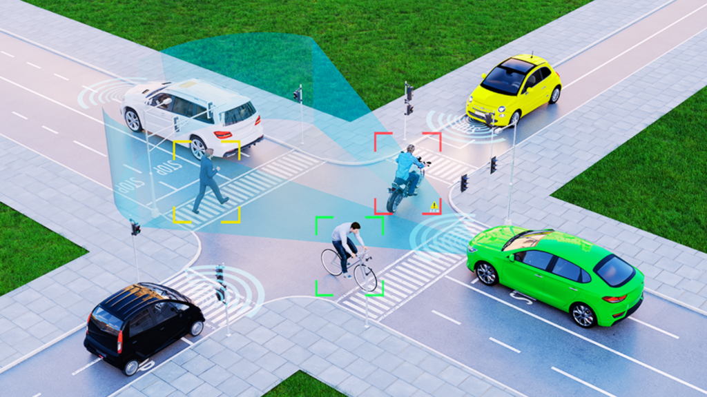
What is Object Tracking in Computer Vision? A Detailed View
Object tracking is a crucial task in computer vision that involves locating and following a specific object in a video or image sequence. It has numerous applications in various fields, including surveillance, robotics, autonomous vehicles, and augmented reality. In this article, we will explore in detail about what is object tracking in computer vision, its importance, and the different techniques used to achieve it. What is Object Tracking in Computer Vision? Object tracking is the process of locating and following a specific object in a video or image sequence over time. It involves identifying the object of interest and then tracking its movement as it moves through the scene. Object tracking is a challenging task due to various factors such as occlusion, illumination changes, and object deformation. Object tracking is an essential task in computer vision as it has numerous applications in various fields. For instance, in surveillance, object tracking is used to monitor the movement of people and vehicles in a particular area. In robotics, object tracking is used to track the movement of objects in a robot’s environment. In autonomous vehicles, object tracking is used to detect and track other vehicles and pedestrians on the road. In augmented reality, object tracking is used to overlay virtual objects on real-world objects. Object Tracking Techniques There are various techniques used to achieve object tracking in computer vision. These techniques can be broadly classified into two categories: model-based and feature-based. Model-based techniques involve creating a model of the object of interest and then tracking it through the scene. The model can be a geometric model, a statistical model, or a combination of both. Geometric models use the object’s shape and size to track it through the scene, while statistical models use the object’s appearance to track it. Feature-based techniques involve identifying and tracking specific features of the object of interest through the scene. These features can be edges, corners, or other distinctive points on the object. Feature-based techniques are more robust to changes in the object’s appearance and are less computationally intensive than model-based techniques. Tpu vs Gpu: The Giants of Computational Power Object Tracking Challenges Object tracking is a challenging task due to various factors such as occlusion, illumination changes, and object deformation. Occlusion occurs when the object of interest is partially or completely hidden by other objects in the scene. Illumination changes occur when the lighting conditions in the scene change, making it difficult to track the object’s appearance. Object deformation occurs when the object changes shape or size, making it difficult to track its movement. Researchers have developed various techniques to overcome these challenges such as multi-object tracking, online tracking, and deep learning. Multi-Object Tracking Multi-object tracking is a technique used to track multiple objects simultaneously in a video or image sequence. It involves detecting and tracking multiple objects in the scene and then associating them over time. Multi-object tracking is a challenging task as it requires tracking multiple objects with different appearances and movements. Online Tracking Online tracking is a technique used to track objects in real-time as they move through the scene. It involves updating the object’s position and appearance as new frames are received. Online tracking is a challenging task as it requires tracking objects in real-time, which can be computationally intensive. Deep Learning Deep learning is a subfield of machine learning that involves training artificial neural networks to perform specific tasks. Deep learning has revolutionized object tracking in computer vision by enabling the development of more accurate and robust object trackers. Deep learning-based object trackers use convolutional neural networks (CNNs) to learn the object’s appearance and motion patterns and then use this information to track the object through the scene. Conclusion Object tracking is a crucial task in computer vision that has numerous applications in various fields. It involves locating and following a specific object in a video or image sequence over time. Object tracking is a challenging task due to various factors such as occlusion, illumination changes, and object deformation. However, researchers have developed various techniques, such as multi-object tracking, online tracking, and deep learning to overcome these challenges and improve the accuracy and robustness of object trackers. With the continued development of computer vision technology, object tracking is expected to become even more accurate and robust, enabling new applications in various fields. References
Python 2 vs Python 3: A Comparative Study

Python 3.0 introduced many changes and improvements compared to Python 2. Some of the biggest differences include the use of Unicode strings by default 6, the removal of some old and deprecated features 4, and changes to the syntax and semantics of the language 4. And do you know that about 50% of programmers prefer coding in Python? Print function: In Python 3.0, the print statement was replaced with a print() function, which has some differences in syntax and behavior. For example, you need to use parentheses around the arguments to print, and you can no longer use the comma to separate arguments or the “>>” syntax to redirect output. Accelerate Your Career in AI with Best Machine Learning Courses Unicode Support Python 3.0 has much better support for Unicode than previous versions of the language, which makes it easier to work with non-ASCII text and internationalization. However, it also requires some changes to how you work with strings and files, so it’s important to be aware of the differences between Python 3.0 and earlier versions. Speed: Python 2 vs Python 3 The speed of Python 3 compared to Python 2 can depend on a variety of factors, including the specific code being run, the version of Python being used, and the implementation of Python (e.g. CPython, PyPy, Jython, etc.). In general, Python 3 is not significantly faster or slower than Python 2 for most tasks, but there are some differences to be aware of: Some tests show Python 3 code executing faster than Python 2, particularly for functions involving complex calculations and large data sets. Comparing Python 2 vs Python 3 in the Realm of AI Training In the realm of AI training, Python 3 is generally considered to be the better choice over Python 2 for several reasons: Overall, while Python 2 is still widely used in some AI applications, Python 3 is generally considered to be the better choice for new projects and for applications that require modern libraries and frameworks. If you are starting a new AI project, it’s recommended to use Python 3 and to take advantage of its improved support for Unicode, type annotations, and asynchronous programming. Best Linux Distro For Programming: Unraveling the Choices References
DALL-E Mini: Too Much Traffic

Artificial Intelligence Generated Content (AIGC) has been gaining much attention in recent years, with large tech companies like OpenAI and Google developing models that can generate text, images, and even music. One of the most impressive AIGC models is DALL-E, which can generate high-quality images from textual descriptions. However, the recent release of DALL-E Mini has caused some concerns about the impact of AIGC on the environment and the internet infrastructure. In this article, we will explore the issue DALL-E Mini: Too Much Traffic, capabilities, its potential impact on the internet, and the ethical considerations of AIGC.OpenShift Vs Kubernetes: A Comprehensive Comparison What is DALL-E Mini? DALL-E Mini is a smaller version of the original DALL-E model, which was introduced by OpenAI in January 2021. DALL-E stands for “Dali + WALL-E”, as the model was trained to generate surrealistic images based on textual descriptions. The original DALL-E model had 12 billion parameters and was trained on a dataset of text-image pairs. It was able to generate a wide range of images, from animals to objects to scenes, with impressive detail and creativity. DALL-E Mini, on the other hand, has only 125 million parameters, which makes it much smaller and faster than the original model. It was released in June 2021 as a way to make the DALL-E technology more accessible to developers and researchers. According to OpenAI, DALL-E Mini can generate images that are “nearly as good” as those generated by the original DALL-E, but with much less computational resources. DALL-E Mini: Too Much Traffic While DALL-E Mini may be a great tool for developers and researchers, it has raised concerns about the impact of AIGC on the internet infrastructure. Generating images with AIGC models requires a lot of computational resources, including GPUs and servers. This means that every time someone uses DALL-E Mini to generate an image, it puts a strain on the internet traffic and the energy consumption of the data centers. According to a recent report by OpenAI, the original DALL-E model consumed about 1.3 GWh of energy during its training, which is equivalent to the energy consumption of about 126 American households in a year. While DALL-E Mini is much smaller and faster than the original model, it still requires a significant amount of energy to generate images. This means that if DALL-E Mini becomes widely used, it could contribute to the already high energy consumption of the internet and the data centers. This could lead to more carbon emissions and environmental impact, as well as higher costs for the companies that operate the data centers. Moreover, the traffic generated by AIGC models like DALL-E Mini could also cause congestion and slow down the internet for other users. This is because the data generated by AIGC models is often large and requires high bandwidth to transfer. If many users are generating images with DALL-E Mini at the same time, it could create a bottleneck in the internet traffic and affect the performance of other applications. AWS vs Azure: The Definitive Comparison The Ethical Considerations Apart from the technical and environmental concerns, the rise of AIGC models like DALL-E Mini also raises ethical considerations about the use of AI in content creation. One of the main concerns is the potential loss of jobs for human creators, as AIGC models can automate the creation of large amounts of content in a short amount of time. This could lead to a displacement of human workers and a concentration of power in the hands of the companies that own the AIGC models. Another concern is the potential misuse of AIGC models for malicious purposes, such as generating fake news, propaganda, or deepfakes. AIGC models can be trained to generate text and images that are indistinguishable from those created by humans, which could be used to spread misinformation or manipulate public opinion. This could have serious consequences for democracy, social cohesion, and individual rights. Conclusion DALL-E Mini is a powerful AIGC model that can generate high-quality images from textual descriptions with much less computational resources than the original DALL-E model. However, its release has raised concerns about the impact of AIGC on the environment, the internet infrastructure, and the ethical considerations of AI in content creation. As AI technology continues to advance, it is important to address these concerns and ensure that AI is used for the benefit of society as a whole. References
Best Algorithms for Face Recognition
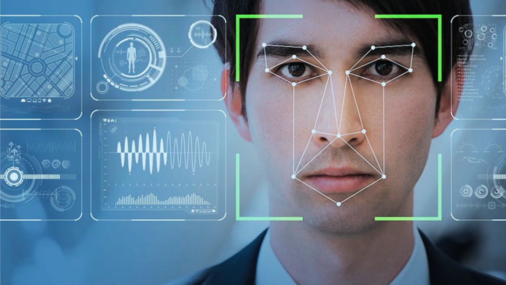
Face recognition is a rapidly growing field in artificial intelligence and computer vision. With the breakthroughs made in deep convolutional neural networks, face recognition has become an important application in the industrial world. In this article, we will explore the best algorithms for face recognition, including their history, pipeline, and evaluation datasets. History of Face Recognition Face recognition has been studied for decades, but it wasn’t until the 1990s that it became a popular research topic. In the early days, face recognition algorithms were based on manually designed features, such as the eigenface method. However, these methods were limited in their ability to handle variations in lighting, pose, and expression. In recent years, deep learning algorithms have revolutionized the field of face recognition. These algorithms use convolutional neural networks to learn features directly from the raw image data. This has led to significant improvements in accuracy and robustness. Bayesian Network vs Neural Network Pipeline in Deep Learning Framework The pipeline in the deep learning framework for face recognition consists of several stages. There are several challenges in each stage of the pipeline. For example, face detection and alignment can be difficult in the presence of occlusions or extreme poses. Feature extraction can be sensitive to variations in lighting and expression. And matching can be challenging when dealing with large databases or unknown faces. Algorithms for Face Recognition There are several algorithms for face recognition, including those based on conventional, manually designed features and those based on deep learning. Some of the most popular algorithms include the following. Eigenfaces This algorithm uses principal component analysis to extract features from the face image. It was one of the earliest algorithms for face recognition and is still used today in some applications. Fisherfaces This algorithm is an extension of eigenfaces that takes into account the class labels of the face images. It has been shown to be more robust than eigenfaces in the presence of variations in lighting and expression. DeepFace This algorithm uses a deep convolutional neural network to extract features from the face image. It was one of the first algorithms to achieve human-level performance on the Labeled Faces in the Wild dataset. FaceNet This algorithm uses a triplet loss function to learn a mapping from face images to a high-dimensional feature space. It has achieved state-of-the-art performance on several face recognition benchmarks, including the LFW, AgeDB, CFP-FP, and IJB-C datasets. Evaluation Datasets Evaluation datasets are an important part of face recognition research. They provide a standardized way to compare the performance of different algorithms. Some of the most popular evaluation datasets include the following. Labeled Faces in the Wild (LFW) This dataset contains more than 13,000 face images of 5,749 people. It is one of the most widely used datasets for face recognition research. AgeDB This dataset contains more than 16,000 face images of 568 people, with age annotations. It is used to evaluate the performance of face recognition algorithms on age-invariant face recognition. CFP-FP This dataset contains more than 7,000 face images of 500 people, with frontal and profile views. It is used to evaluate the performance of face recognition algorithms on unconstrained face recognition. IJB-C This dataset contains more than 31,000 face images of 1,845 people, with varying levels of pose, illumination, and occlusion. It is used to evaluate the performance of face recognition algorithms on unconstrained face recognition. Conclusion In conclusion, face recognition is a rapidly growing field in artificial intelligence and computer vision. With the breakthroughs made in deep convolutional neural networks, face recognition has become an important application in the industrial world. In this article, we explored the best algorithms for face recognition, including their history, pipeline, and evaluation datasets. FAQs References
Overview of Neural Radiance Fields (NeRF)
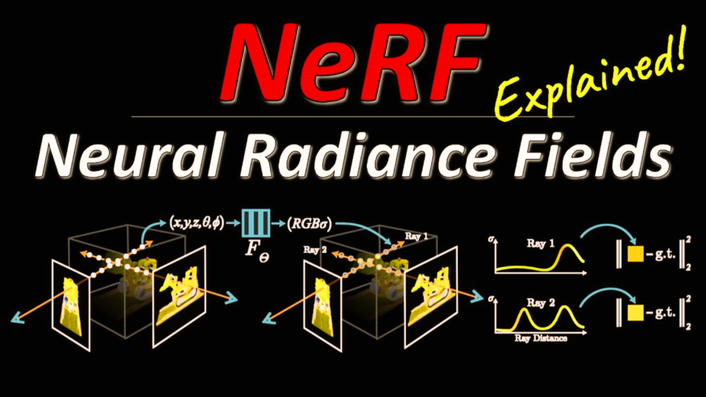
Understanding NeRF: The Neural Radiance Fields NeRF is an acronym for Neural Radiance Fields, an AI-based approach to 3D image rendering. The crux of this model lies in its ability to use a neural network to learn. It can learn a continuous volumetric scene function from a sparse set of 2D images. Bayesian Network vs Neural Network This function maps a 3D spatial location (along with a 2D viewing direction) to a color and opacity. This results in highly detailed and photorealistic 3D structures. The Intriguing Story Behind NeRF The development of NeRF was a response to the challenges of 3D rendering. The traditional methods, while effective, were computationally intensive. That’s because the resulting images often lacked photorealistic details. These limitations spurred researchers at Google Research to propose a novel approach—NeRF. The NeRF paper, titled “NeRF: Representing Scenes as Neural Radiance Fields for View Synthesis,” was released in March 2020. The paper elaborated on how NeRF deploys a fully connected deep network (a Multilayer Perceptron). It discusses how NeRF uses Multilayer Perceptron to model the volumetric scene. It introduced a technique that drastically reduced the computation required for rendering. And thus, it is improving the quality of the 3D structures produced. Why is NeRF Famous? NeRF garnered attention in the AI community due to its novel approach to a long-standing challenge. The system’s capability to produce high-quality, detailed 3D models from a small set of 2D images was groundbreaking. NeRF’s fame can be attributed to several of its attributes. Firstly, it delivers exceptional detail by modeling fine structures and complex illumination effects such as reflections and shadows. Secondly, NeRF significantly cuts down the computational cost associated with traditional 3D rendering. Lastly, its flexibility enables it to handle various scene types, including indoor and outdoor environments. This feature perfectly works for both artificial and natural structures. The Global Impact of NeRF: Which Country Made It? NeRF is universally applauded but its creation can be credited to researchers from Google Research in the United States. Their ground-breaking work has revolutionized 3D image rendering. In doing so, it has inspired researchers worldwide to explore new applications and enhancements to the technology. The Significance of the NeRF Paper The NeRF paper is pivotal in the world of AI and computer vision. It is in this document that the method of leveraging neural networks for 3D rendering was first proposed. The paper meticulously presents the innovative process. It starts from the construction of the neural network to the techniques used for sampling and optimizing the model. The NeRF paper holds a significant place in AI literature due to the radical shift it proposes in the methodology for 3D rendering. The novel approach, combined with the potential for wide-ranging applications, makes the paper a must-read for anyone. It’s groundbreaking for people involved in AI computer vision, and 3D rendering. Conclusion The development of Neural Radiance Fields (NeRF) represents a significant step forward in the field of 3D image rendering. Its unique methodology uses AI to transform a small set of 2D images into highly detailed, photorealistic 3D structures. And thus, it’s fundamentally changing the way we approach 3D rendering. Despite its newness, NeRF continues to make waves in the AI community, inspiring new research. The journey of NeRF, as detailed in the NeRF paper, showcases how innovative thinking can be coupled with AI. It can revolutionize established processes and open new avenues for technological advancement. References
Bounding Boxes in Computer Vision
A New Scheme for Training Object Class Detectors Using Only Human Verification! Object class detection is a central problem in computer vision. It involves identifying and localizing objects of interest in an image. One of the most common methods for training object class detectors is through the use of bounding-box annotations. However, manually drawing bounding-boxes is a tedious and time-consuming task. In this article, we introduce a new scheme for training object class detectors using only human verification, which eliminates the need for manual bounding-box annotations. Electric Car Efficiency vs Gas: A Comprehensive Comparison The Problem with Bounding-Box Annotations Bounding-box annotation is a crucial step in training object class detectors. It involves drawing a rectangle around an object of interest in an image. This process is repeated for every object in the training set, resulting in a large number of bounding-box annotations. However, manually drawing bounding-boxes is a time-consuming and expensive task. It requires a lot of human effort and can take weeks or even months to complete. The Proposed Scheme To address the problem of manual bounding-box annotations, we propose a new scheme for training object class detectors using only human verification. Our scheme involves three steps: re-training the detector, re-localizing objects in the training images, and human verification. The verification signal is used to improve re-training and to reduce the search space for re-localization, which makes these steps different from what is normally done in a weakly supervised setting. The Benefits of Using Human Verification Using human verification in the training process has several benefits. Other Ways to Reduce Annotation Effort In addition to our proposed scheme, there are other ways to reduce annotation effort. Some authors have tried to learn object detectors from videos, where the spatio-temporal coherence of the video frames facilitates object localization. An alternative is transfer learning, where learning a model for a new class is helped by labeled examples of related classes. Other types of data, such as text from web pages or newspapers or eye-tracking data, have also been used as a weak annotation signal to train object detectors. Experiments and Results We conducted extensive experiments on PASCAL VOC 2007 to evaluate the effectiveness of our proposed scheme. The results showed that our scheme delivers detectors performing almost as good as those trained in a fully supervised setting, without ever drawing any bounding-box. Moreover, our scheme substantially reduces total annotation time by a factor of 6×-9×. These results demonstrate the effectiveness of our proposed scheme in reducing the cost and time required for training object class detectors. Human-Machine Collaboration Approaches Human-machine collaboration approaches have been successfully used in tasks that are currently too difficult to be solved by computer vision alone. These approaches combine the responses of pre-trained computer vision models on a new test image with human input to fully solve the task. In the domain of object detection, Russakovsky et al. propose such a scheme to fully detect all objects in images of complex scenes. Importantly, their object detectors are pre-trained on bounding-boxes from the large training set of ILSVRC 2014, as their goal is not to make an efficient training scheme. Conclusion In conclusion, the use of bounding-box annotations in computer vision is a crucial step in training object class detectors. However, manually drawing bounding-boxes is a tedious and time-consuming task. Our proposed scheme for training object class detectors using only human verification eliminates the need for manual bounding-box annotations, which saves time and reduces the cost of training object class detectors. Moreover, our scheme delivers detectors performing almost as good as those trained in a fully supervised setting, without ever drawing any bounding-box. As the verification task is very quick, our scheme substantially reduces total annotation time by a factor of 6×-9×. This new scheme for training object class detectors using only human verification is a promising direction for future research in computer vision. FAQs References
Overfitting vs Underfitting: Difference Explained
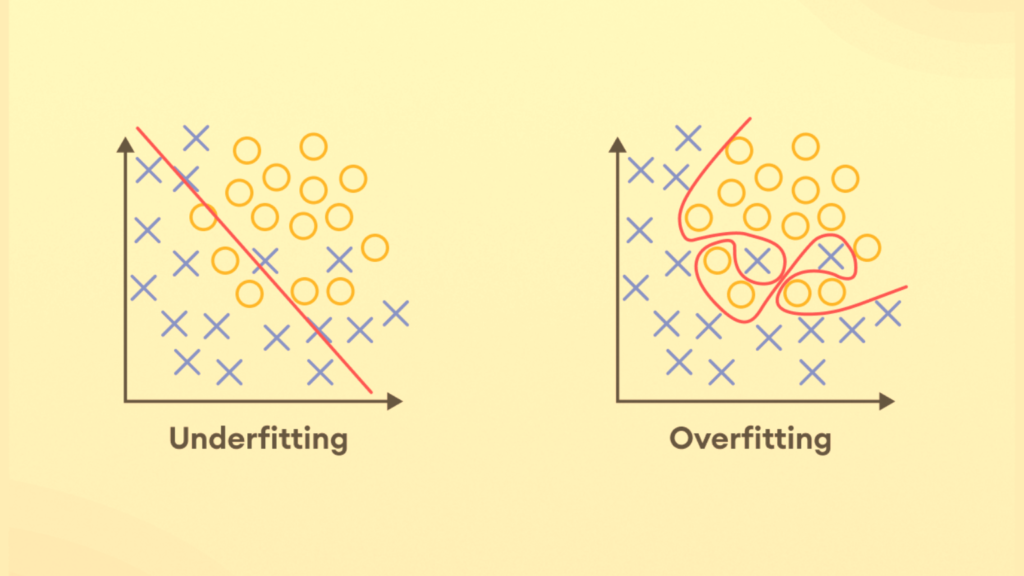
Overfitting and underfitting are the twin hurdles that every Data Scientist, rookie or seasoned, grapples with. While overfitting tempts with its flawless performance on training data only to falter in real-world applications, underfitting reveals a model’s lackluster grasp of the data’s essence. Achieving the golden mean between these two states is where the art of model crafting truly lies. This blog post discusses the intricacies that distinguish overfitting from underfitting. Let’s demystify these model conundrums and equipping ourselves to navigate them adeptly. Overfitting in Machine Learning: An Illusion of Accuracy Overfitting occurs when an ML model learns the training data too well. It happens when a machine learning model captures all its intricacies, noises, and even outliers. The result is an exceedingly complex model that performs exceptionally well on the training data. But there’s a huge downfall, such a model fails miserably when it encounters new, unseen data. What is an example of an Overfitting Model? Consider an example where you are training a model to predict house prices. It’s predicting prices based on features such as area, number of rooms, location, etc. An overfit model in this scenario would learn the training data to such an extent that it might start considering irrelevant or random features. If it’s considering features like the house number and the color of the exterior, it’s of no use. Considering the importance and thinking that they may influence the price is not good. Such a model may seem incredibly accurate with the training data. But when it’s used to predict the prices of new houses, its performance will likely be poor. This is because the irrelevant features it relied upon do not actually contribute to the price of a house. Underfitting in Machine Learning: Oversimplification Underfitting is almost the opposite of overfitting. It occurs when an ML model is too simple to capture the underlying patterns in the data. An underfit model lacks the complexity needed to learn from the training data. Hence, it fails to capture the relationship between the features and the target variable adequately. Since the model is failing to consider all the factors, it becomes useless. What is an example of an Underfitting Model? Let’s revisit the house pricing example. If the model is underfitting, it might ignore significant factors. These include the area or location, and it may predict house prices solely based on the number of rooms. Such a simplistic model would perform poorly on both the training and testing data. And the main reason is that it fails to capture the complexity of real-world pricing factors. Overfitting vs Underfitting: The Battle of Complexity In essence, the battle of underfitting vs overfitting in machine learning is a trade-off between bias and variance. Simply put, it’s a trade-off between oversimplification and excessive complexity. An underfit model suffers from high bias; it consistently misses important trends. On the other hand, an overfit model has high variance. It is highly sensitive to the training data and performs poorly on unseen data. Overfitting and Underfitting with Examples To put the concept of overfitting vs underfitting in context, imagine trying to fit a curve to a set of data points. The goal of an ideal model is to find a balance. It should be complex enough to capture the trend, yet not too complex to follow every noise or outlier. After all, the goal of machine learning is not to memorize training data but to generalize well to unseen data. Conclusion Overfitting and underfitting are significant challenges in machine learning. By understanding these concepts, one can better design and tune models to avoid these pitfalls. Measures such as cross-validation, regularization, and ensemble methods can help strike a balance between complexity and simplicity. The goal should be to optimize the model’s ability to learn from the past and predict the future. References
Difference Between Statistics and Machine Learning

In the study of biological systems, two major goals are inference and prediction. Inference creates a mathematical model of the data-generation process to formalize understanding or test a hypothesis about how the system behaves. Prediction, on the other hand, finds generalizable predictive patterns. Both statistics and machine learning can be used for both inference and prediction, but they differ in their approaches and applications. Classical Statistics vs. Machine Learning Classical statistics draws population inferences from a sample. It is designed for data with a few dozen input variables and sample sizes that would be considered small to moderate today. In this scenario, the model fills in the unobserved aspects of the system. Classical statistical modeling makes strong assumptions about data-generating systems, such as linearity, normality, and independence. It is effective when the data are gathered with a carefully controlled experimental design and in the absence of complicated nonlinear interactions. Machine learning, by contrast, concentrates on prediction by using general-purpose learning algorithms to find patterns in often rich and unwieldy data. Machine learning methods are particularly helpful when one is dealing with ‘wide data’, where the number of input variables exceeds the number of subjects, in contrast to ‘long data’, where the number of subjects is greater than that of input variables. Machine learning makes minimal assumptions about the data-generating systems; they can be effective even when the data are gathered without a carefully controlled experimental design and in the presence of complicated nonlinear interactions. However, despite convincing prediction results, the lack of an explicit model can make machine learning solutions difficult to directly relate to existing biological knowledge. Inferential Statistics vs Descriptive Statistics: A Comparative Study Simulation of Gene Expression To compare traditional statistics to machine learning approaches, a simulation of the expression of 40 genes in two phenotypes (-/+) was conducted. Mean gene expression differed between phenotypes, but the simulation was set up so that the mean difference for the first 30 genes was not related to phenotype. The last ten genes were dysregulated, with systematic differences in mean expression between phenotypes. Using these average expression values, an RNA-seq experiment was simulated in which the observed counts for each gene were sampled from a Poisson distribution with mean exp(x + ε), where x is the mean log expression, unique to the gene and phenotype, and ε ~ N(0, 0.15) acts as biological variability that varies from subject to subject. Difference Between Statistics and Machine Learning In the simulation of gene expression, classical statistical methods and machine learning methods were compared. For classical statistical methods, a two-sample t-test was used to compare the mean expression of each gene between the two phenotypes. For machine learning methods, a random forest classifier was used to predict the phenotype based on the expression of all 40 genes. The results showed that both classical statistical methods and machine learning methods were able to identify the dysregulated genes with high accuracy. However, the classical statistical methods were only able to identify the dysregulated genes because they were pre-selected based on prior knowledge. In contrast, the machine learning methods were able to identify the dysregulated genes without any prior knowledge by considering all 40 genes simultaneously. The Importance of Feature Selection One of the challenges of machine learning is feature selection, or identifying which input variables (genes) are most important for predicting the output variable (phenotype). In the simulation of gene expression, the random forest classifier was able to identify the dysregulated genes as the most important features for predicting the phenotype. However, it is important to note that not all dysregulated genes were identified as important features, and some non-dysregulated genes were identified as important features. This highlights the importance of careful feature selection in machine learning, as well as the potential for machine learning to identify novel biomarkers that may not be identified using classical statistical methods. Best Practices For Machine Learning Applications Conclusion In conclusion, both classical statistical methods and machine learning methods have their strengths and weaknesses in the study of biological systems. Classical statistical methods are effective when the data are gathered with a carefully controlled experimental design and in the absence of complicated nonlinear interactions. Machine learning methods are effective when dealing with ‘wide data’ and complicated nonlinear interactions, but may be difficult to directly relate to existing biological knowledge. The simulation of gene expression showed that both classical statistical methods and machine learning methods were able to identify dysregulated genes with high accuracy. However, machine learning methods were able to identify dysregulated genes without any prior knowledge, by considering all genes simultaneously. This highlights the potential for machine learning to identify novel biomarkers that may not be identified using classical statistical methods. Overall, the choice of statistical method or machine learning method should depend on the specific research question and the characteristics of the data being analyzed. By understanding the strengths and weaknesses of both approaches, researchers can make informed decisions about which method to use in their research. FAQS References
HDFS vs S3: Understanding the Differences, Advantages, and Use Cases
HDFS is a distributed file system designed to manage large data sets spanning multiple nodes. It is a key component of the Apache Hadoop ecosystem. HDFS provides high-throughput access to application data and is designed to handle failures gracefully. On the other hand, S3, provided by Amazon Web Services (AWS), is an object storage service. It offers industry-leading scalability, data availability, security, and performance. Thus, it enables customers to store and protect any amount of data for a range of use cases. Is HDFS Faster Than S3? A commonly asked question is: “Is HDFS faster than S3?” The answer, like many things in the big data world, is: it depends. HDFS, being a distributed file system, is designed to provide high-throughput access to data. Especially, when the data and the compute nodes are on the same cluster. This proximity can provide faster data access times. Conversely, S3, being an object store, may experience latency due to the separation of storage and compute resources. However, with recent advancements in AWS technologies, this latency has been minimized. Can We Replace HDFS with S3? Another question often posed is, “Can we replace HDFS with S3?” The answer primarily hinges on your specific use case. S3 can be a suitable HDFS alternative for storing large amounts of data. It becomes more suitable when used in conjunction with other AWS services. It provides durability, ease of use, and excellent scalability, which might be beneficial in various scenarios. However, in cases where data locality is crucial HDFS might still be the better option. For instance, running iterative algorithms on a Hadoop cluster. Additionally, HDFS allows for more straightforward data replication strategies, which is essential in disaster recovery scenarios. Is HDFS an Object Store? Now let’s tackle the question, “Is HDFS an object store?” In short, no, it isn’t. HDFS is a block storage system that splits data into multiple blocks. It then distributes them across the nodes in a cluster. Unlike object stores like S3, which handle data as objects, HDFS stores data in a filesystem hierarchy. That’s why it is considered ideal for handling large files. Can S3 be Used for Big Data? “Can S3 be used for big data?” is another query we encounter. The answer is a resounding yes. Amazon S3 is built to store and retrieve any amount of data at any time, from anywhere. Its durability and availability make it a compelling choice for big data workloads. Furthermore, it offers a wide array of integrations with big data frameworks like Apache Spark and Hadoop. Is S3 an Object Store? The answer to “Is S3 an object store?” is yes. Amazon S3 is designed to store and retrieve any amount of data at any time. It treats data as objects, and these objects are stored in buckets. Each object contains both data and metadata and is identified by a unique, user-assigned key. Is HDFS a Block Storage? When we question, “Is HDFS a block storage?” the answer is yes. HDFS splits large data sets into smaller blocks, usually of size 64MB or 128MB. It then distributes these across multiple nodes in a Hadoop cluster. This design allows for faster processing of large data sets as multiple nodes can process different blocks concurrently. Electric Car Efficiency vs Gas: A Comprehensive Comparison HDFS vs S3: The Final Verdict When comparing HDFS vs S3, it’s crucial to understand that each storage system has its strengths and weaknesses. They both are designed for different scenarios and different purposes. HDFS shines in environments where data locality and replication are key. Whereas S3 stands out for its scalability, durability, and integration with other AWS services. Lastly, addressing the question “Is S3 HDFS?” it is important to note that S3 and HDFS are two dihttps://jonascleveland.com/electric-car-efficiency-vs-gas/stinct storage systems. And of course, each has its unique attributes and uses. There is, however, an HDFS-S3 connector available to bridge these technologies. It provides the ability to leverage the benefits of both systems in a unified big data solution. Conclusion whether you choose HDFS or S3, it largely depends on your specific use case. Both offer unique benefits, and understanding these will help guide you in your big data journey. Always consider factors such as data volume, required processing speed, cost, and specific workload requirements before making a choice between HDFS and S3. References
Bayesian Network vs Neural Network
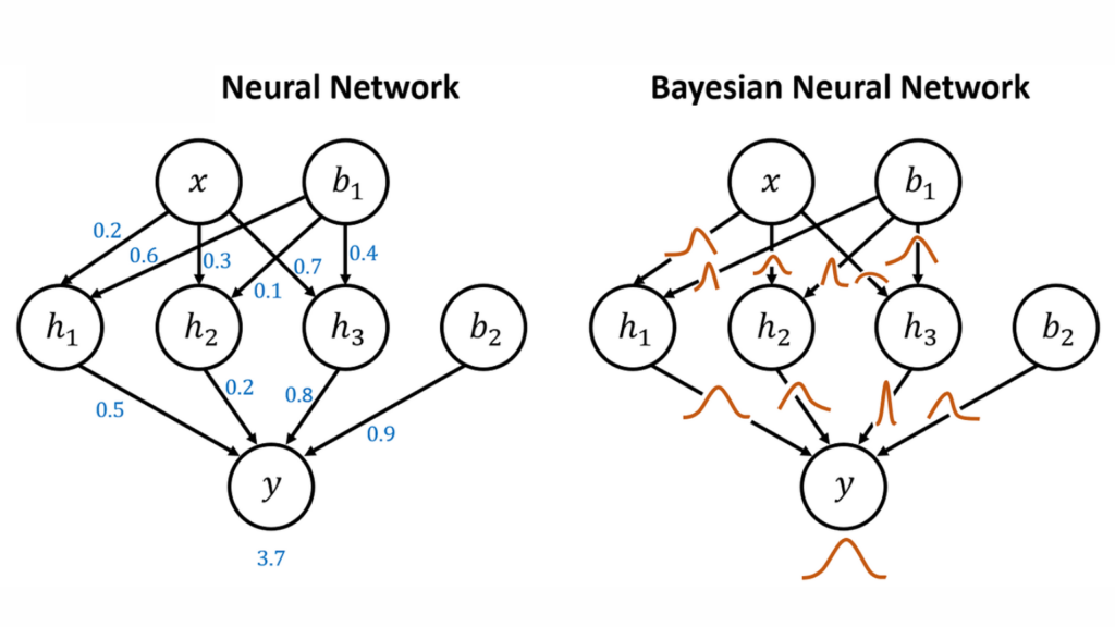
A Bayesian Network is also known as a belief network or directed acyclic graphical model. It is a probabilistic graphical model that represents a set of variables and their conditional dependencies via a directed acyclic graph (DAG). In simpler terms, Bayesian networks are mathematical models that represent the relationships among variables. In doing so, it helps in predicting outcomes based on input data. On the other hand, a Neural Network, inspired by biological neurons, is a computing system. It consists of highly interconnected nodes or “neurons” that process information. They process information by responding to external inputs and relaying information between each unit. Neural Networks are designed to classify and pattern information in a manner similar to the human brain. So, the key difference lies in their operational mechanisms: Bayesian Networks employ probabilistic relationships. Whereas Neural Networks rely on learning patterns in data through complex, neuron-like structures. Is a Bayesian Network a Neural Network? Given their differing natures, it would be incorrect to categorize Bayesian Networks as a type of Neural Network. They are distinct models with unique theoretical foundations. However, in certain situations, the techniques can be merged to create a Bayesian Neural Network, an intriguing fusion that we will discuss later in this article. What is the difference between Machine Learning and Bayesian Networks? Machine Learning is a broad field of study and application that encompasses numerous methods and models, including Bayesian Networks. It aims to build systems that can learn from data, improve over time, and make decisions or predictions. A Bayesian Network, on the other hand, is a specific tool used within the field of machine learning. It is designed to model uncertain knowledge and reasoning.Electric Car Efficiency vs Gas: A Comprehensive Comparison What is the difference between a Random Forest and a Bayesian Network? Random Forests and Bayesian Networks are both powerful machine-learning techniques but have different approaches. A Random Forest is an ensemble learning method that operates by constructing multiple decision trees. It outputs the mode of the classes for classification or mean prediction for regression. It is often used for its simplicity and ability to handle large datasets with high dimensionality. In contrast, a Bayesian Network is a probabilistic graphical model that uses Bayes’ theorem to infer the probabilities of uncertain events. It shines in applications where relationships among features need to be modeled explicitly or where interpretability is critical. What is the difference between Naïve Bayes and Bayesian Networks? Naïve Bayes is a simplified version of a Bayesian Network. In Naïve Bayes, all features are assumed to be independent of each other, an assumption that is “naïve” in many real-world situations. On the contrary, a Bayesian Network represents dependencies among all variables and does not necessarily assume independence, providing a more realistic and complex modeling approach. Bayesian Neural Network Now let’s discuss the intriguing hybrid of the two methods we mentioned earlier – the Bayesian Neural Network. This model integrates the complexity and learning capacity of a Neural Network with the probabilistic approach of a Bayesian model. A Bayesian Neural Network captures the uncertainty in its predictions by providing a distribution of outcomes rather than a single-point estimate. This feature makes Bayesian Neural Networks highly useful in tasks where estimation of uncertainty is crucial. This means you can use it for financial forecasting or medical diagnosis. Bayesian Neural Network Example Consider a Bayesian Neural Network deployed for predicting stock market trends. Unlike a regular Neural Network that might predict a specific value, a Bayesian Neural Network would give a range of potential values with associated probabilities. This feature is particularly useful for traders, who could not only gain insight into expected trends but also understand the inherent uncertainty in these predictions. Bayesian Neural Network for Classification In a classification task, a Bayesian Neural Network provides the probabilities for each class, allowing for a more nuanced understanding of the results. This can be particularly useful when working with imbalanced datasets, where misclassification costs may vary among classes. Bayesian Neural Network Tutorial Delving into the step-by-step details of building a Bayesian Neural Network is beyond the scope of this article. Resources such as the TensorFlow Probability library provide extensive documentation and tutorials for those interested in implementing this innovative hybrid model. Conclusion Bayesian Networks and Neural Networks are distinct models with unique advantages and applications. Their fusion into a Bayesian Neural Network opens up new possibilities for modeling uncertainty in complex predictive tasks. As the field of machine learning continues to evolve, the understanding and application of these models will continue to be an essential aspect of any data scientist’s toolkit. References